Voight-Kampff Test #2

VK 検査についての 2 ポスト目。Wiki によると、「デッカードとタイレルの会話において、レプリカントであるか否かを判定するためには通常20～30項目の質問が必要になる、と述べられているが、レイチェルがレプリカントであることを判定するには100項目以上の質問が必要であった」そうなのですが、これってどういうことなんでしょうか。

まず、VK 検査で使われる機材ですが、基本的には嘘発見器/ポリグラフみたいなもののようです。「この時代に生きる人間の感情を大きく揺さぶるような質問を繰り返し、それに対して起きる肉体的反応を計測することで、対象が人間かレプリカントであるかを判別することができる、とされている」とか、"It measures bodily functions such as respiration, blush response, heart rate and eye movement in response to questions dealing with empathy" とか言われています。

では、具体的にどういう検査をしているのでしょうか。まず、最終的には yes/no の判定をしているので、帰無仮説検定のような統計推論を行っている可能性が高いのではないでしょうか (ベイズでも、BF がある一定値を超えたらレプリカントと判定しているのでは？)。映画のシーンを見ると、共感条件 (感情を大きく揺さぶる質問の条件) と統制条件が設けられているわけではなく、共感条件しかないようです (項目は cross-referenced になっているとデッカードが言っているので、なんだかもっとややこしそうですが、それは考えないことにします)。ということは通常の人間であればこれくらいの値を示すだろうという基準値があり、それと比較して、この程度の値であればレプリカントだと判定するのではないかと思います。なので one-sample t test に近いのではないかと推測してみましょう。

しかしいずれせによ、映像を見ていると、なんだか1項目ずつ尋ねていって、有意差が出たら「あんたレプリカントやね」と判定してしまっている感がぬぐえません。ここで 再現可能性問題に敏感な人はすぐ思い当るかもしれませんが、これは典型的な QRPs のひとつに数えられる行為です。普通の心理学実験の場合だったら、参加者をひとり足しては検定をかけ、またひとり足しては検定をかけ、またひとり... と続けていって、有意になったところで「おりゃ結果出たぜ！」と叫んですぐ論文にしてしまう、というやり方になるわけで、これをやると、第一種の過誤 (本当は効果が無いにも関わらず、あると報告してしまうこと) の確率が飛躍的に上がってしまうため、やっちゃダメと言われている行為、つまり p hacking の一種なのです。

ではデッカードも第一種の過誤を犯して、本当はレプリカントでもない人間を引退させたり (aka 殺したり)しているのでしょうか？ なお、ここで注意して欲しいのは、これは先のポストで話した事前確率云々の話とは別で、検定自体に関わる問題ですから、デッカードがいかに事前捜査で事前確率を高めて検査に臨んだとしても生じてしまう問題です。

というわけで R でシミュレーションをやってみましょう (というのは言い訳で、単に僕がシミュレーションの練習をしたかっただけです。あと、こんなの解析解出るじゃんか、と言われたらそうなんですが、すいません、数学苦手なので...)。なお、僕は R プログラミングは本当に初心者なので、その道のプロである中京心理の高橋先生にアドバイスいただきました。みなさんもプログラミング上達したいのなら中京心理に来てください。一緒に勉強しましょう！

さてシミュレーションの中身ですが、前提として、まずデッカードは one sample t test をやっていることにします。人間の反応値の平均を効果量ゼロとして、そこから VK 検査の値が有意に外れていたら、レプリカントだと判定することにします。ここで第一種の過誤が起こるのは、検査対象の人が実は人間だった場合ですから、その場合は効果量ゼロとなります。その他にも、効果量を Cohen's d で言って 0.3, 0.5, 0.8, 1.0 の条件と、あとかなり大きな効果量 1.9 の場合も考えてみることにしましょう (なぜこの値なのかは後で説明します)。ちなみに計測値の分散は単純化して、 SD = 1 の正規分布であることにします。デッカードはバリバリ p hacking をやっていて、一回ずつの検査ごとに検定をかけていき、有意差が出た時点で「あんたレプリカント」判断をしてしまう設定にします。ここで問題になるのが、有意水準をどうするかです。有意水準とは、第一種の過誤のレベルをどのくらいに抑えるか、つまりエラーコントロールをどの程度やるか、についての水準なわけですが、先のポストで述べたように、人間をレプリカントに間違えたら大変なことになるので、おそらくブレードランナーたちは 5 sigma くらいの厳しい基準を設けていると思われます。なのでその条件と、あと比較対象として、今僕たち普通の心理学者が採用している α  = .05 の場合の、2種類を試してみましょう。こういう前提のもとで、1,000人を対象に検査をやった時に、あるトライアルで有意差がでる確率を求めてみます。

で、結果がこちら。

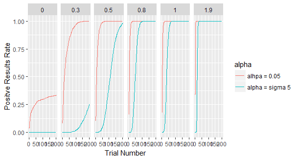効果量6つに応じて、グラフが6つに分かれており、x 軸はトライアル数を示しています。つまり x 軸沿いに右に行くにしたがって、何度も何度も検査を繰り返しているということ。y 軸はそのトライアルの時に「あんたレプリカント」と判断してしまう確率を示しています (i.e. 1,000回中何回そう判断したかの確率)。赤い線は有意水準が心理学者御用達の .05 の場合、青い線は素粒子物理学者御用達の 5 sigma の時です。

左端に注目してください。ここが効果量ゼロ、つまり本当は人間だった時ですね。ところが赤い線を見てみると、けっこうな確率で無益な殺生が繰り返されてしまうことがよく分かります。拡大してみましょう。

一見してやばいですね。赤い線が血の色にしか見えません。仮に我らがブレードランナーたちが慈悲深くて、まあ20試行くらいまでは判断を待ってやるか(・ω・)と思っていたとしても、5回に1回は無実の人間が血祭りにあげられてしまいます。

しかし先のブログで現実的と考えた 5 sigma の基準、つまり青い線を見てみると、どれだけトライアルを重ねてもほぼゼロのまま、つまり無実の人間はほぼひとりも殺されていないことがよく分かります。心理学ではなくて素粒子物理学の教育を受けた人間をブレードランナーに雇うべきだということが如実に分かる結果です。

また、上のグラフと検定力のグラフを比較してみるのも興味深いところです。

こちらは p hacking の前提を考えず、単に何トライアル重ねたら、どのくらいの確率で効果が発見できるかを示したデータで、黒い横線2本は、検定力の基準としてよく勧められる 80% と 95% を示しています。

当たり前ですが、もともと効果ゼロの左端の条件では、有意水準、すなわち第一種の過誤のコントロール水準である .05 と 5 sigma に赤い線、青い線が来ているのが分かります (だから本当はこれらを検定力とは呼べないことに注意してください)。この結果と、上の p hacking をした時の結果を見比べると、α = .05 で p hacking をすると、第一種の過誤の発生確率がどんなことになってしまうのか、よく分かるかと思います。他にも、効果量 0.3 あたりだと、p hacking をした場合、全体的に効果量の見積が大きくなってしまうことがよく分かると思います。仮にちゃんと効果があった場合でも、報告される効果量の見積がインフレを起こしてしまうわけです。

最後に、「レプリカントであるか否かを判定するためには通常20～30項目の質問が必要になる」という記述から、その場合どのくらいの効果量が推定されるのかを見てみましょう。まあ有意水準 5 sigma だと p hacking してもしていなくてもそう変わらなさそうなので、単純に R の検定力分析のパッケージで、20試行で有意水準 5 sigma、検定力 80% を達成できるのは、どのくらいの効果量なのかを調べてみると、d = 1.91 くらいと出ました。検定力のグラフで見てみると次のような感じです。

確かに20試行目くらいで 80% 検定力を達成しています。しかしそれにしても、通常 d = .8 で大きな効果と言われるわけですから、めちゃくちゃでかい効果であることが分かります。おそらく VK 検査はとてつもなく精確な測定なのでしょう (映像ではまったくそうは見えませんが、たぶん未来はなんかすごいんですよ)。

そうなると気になるのが「レイチェルがレプリカントであることを判定するには100項目以上の質問が必要であった」という記述です。こちらも同じ基準で、試行数だけ100に変えて調べてみると、d = 0.62 くらい。検定力グラフで見ると下のふたつの中間くらいだろうと思われます。普通のレプリカントとレイチェルがどれだけ違っていたのか、よく分かりますね。

結論。デッカードたちが 5 sigma の基準を使っており、さらに VK 検査が実は異常な精度を誇る未来の超技術なのだと考えれば、p hacking してても、人間を間違えて殺す可能性はほとんど無いだろう、ということになるかと思います。他方、5% 有意水準ではガンガン冤罪処刑が行われることになるわけですから、心理学者には VK 検査やらしちゃ駄目ですね、というお話でした。

以下コードです。統計解釈や記述方法など、間違っていたら是非教えてください。

	# The below code is to check unavilable packages
	# and install them automatically
	# Create a variable for the requird packages
	requiredPackages <- c("tidyverse")
	# Create a variable for the required but missing packages
	# "installed.packages()[, "Packages"]" shows
	# only the names of installed packaes with no other unnecessary information.
	newPackages <- requiredPackages[!(requiredPackages %in% installed.packages()[, "Package"])]
	# The next code says if there's something in "new.packages" then
	# install "new.packages".
	if(length(newPackages)) install.packages(newPackages)
	#################################################
	library(tidyverse)
	set.seed(1)
	#################################################
	# What's the power of one sample t test in each trial?
	# first, creaat the full combinations of effect size and respnose number.
	powerData <- expand.grid(es = esCondVector, resN = resNVector)
	# eliminate the trials with only one response
	powerData <- as.data.frame(filter(powerData, resN != 1))
	# Here is a function to calculate power of one sample t tests
	# with alpha = 0.05
	powerTest5 <- function (x) {
	tentativePowerTest <- power.t.test(n = x$resN, delta = x$es, type = "one.sample", alternative = "one.sided", sig.level = 0.05)
	return(tentativePowerTest$power)
	}
	# Here is another function to calculate power of one sample t tests
	# with alpha = simga5
	powerTestSigma5 <- function (x) {
	tentativePowerTest <- power.t.test(n = x$resN, delta = x$es, type = "one.sample", alternative = "one.sided", sig.level = 1-pnorm(5))
	return(tentativePowerTest$power)
	}
	# apply the functions to all the data.
	powerData$power5 <- powerTest5(powerData)
	powerData$powerSigma5 <- powerTestSigma5(powerData)
	# transform poserData into a long-data form
	powerData <- gather(data = powerData, key = alpha, value = power, c(power5, powerSigma5), factor_key = TRUE)
	# prepare the facet names
	levels(powerData$alpha) <- c("alhpa = 0.05", "alpha = sigma 5")
	# Draw figures
	ggplot(data = powerData, aes(x = resN, y = power, color = factor(alpha)))+
	geom_line() +
	geom_hline(yintercept = c(0.8, 0.95)) +
	facet_grid(. ~ es) +
	labs(x = "Trial Number", y = "Power", color = "alpha")
	# How large will the effect size be for detecting the diffrence between
	# a human an replicant at n = 20 and alpha = sigma 5, power = 0.8?
	power.t.test(n = 20, sd = 1, sig.level = 1-pnorm(5), power = 0.8, type = "one.sample", alternative = "one.sided")
	# Draw figures for es = 1.9 i.e. normal replicants.
	ggplot(data = powerData[powerData$es == 1.9,], aes(x = resN, y = power, color = factor(alpha)))+
	geom_line() +
	geom_hline(yintercept = c(0.8, 0.95)) +
	facet_grid(. ~ es) +
	labs(x = "Trial Number", y = "Power", color = "alpha")
	# How about Rachael with n = 100?
	power.t.test(n = 100, sd = 1, sig.level = 1-pnorm(5), power = 0.8, type = "one.sample", alternative = "one.sided")
	# Draw figures for es = 0.5 & 0.8 i.e. approximtely for Rachael.
	ggplot(data = powerData[powerData$es == c(0.5, 0.8),], aes(x = resN, y = power, color = factor(alpha)))+
	geom_line() +
	geom_hline(yintercept = c(0.8, 0.95)) +
	facet_grid(. ~ es) +
	labs(x = "Trial Number", y = "Power", color = "alpha")
	#################################################
	# Next, let's see the type I error rate.
	# Firstly, creat all responses from a replicant,
	# from which each concrete responses will be sampled
	# to creat cumulative response sets.
	# set the range of effectsize, which could vary among replicants.
	esCondVector <- c(0, 0.3, 0.5, 0.8, 1.0, 1.9)
	# set the number of replicants to 1,000 which will be tested
	# at each effect size.
	nInEsCondVector <- 1:1000
	# set the number of responses taken from a replicant to 150.
	resNVector <- 1:200
	# Creat all combinations of effect size, n in each effect size condition,
	# and response number.
	resData = expand.grid(es = esCondVector, nInEsCond = nInEsCondVector, resN = resNVector)
	# Generate values for each responses from normal distribution
	# with specific effect sizes
	resData$resValue = rnorm(nrow(resData), mean = resData$es, sd = 1)
	# a function for calculating mean, SD, t value, Cohen's d, NHST results
	cumulativeTTest <- function(x) {
	# add a column of effect size to the output
	es <- x$es
	# count the number of response per effect size * number in each ES condition
	resN <- 1:nrow(x)
	# calculate cumulative means
	resMean <- sapply(resN, function(i) {mean(x$resValue[1:i])} )
	# calculate the cumulative SDs
	resSd <- sapply(resN, function(i) {sd(x$resValue[1:i])} )
	# create a data frame of the calculated values
	tentativeResData <- data.frame(es, resN, resMean, resSd)
	# create and add statistical values
	tentativeResData <- mutate(tentativeResData,
	tValue = (resMean - 0)/(resSd/sqrt(resN)),
	pValue = pt(tValue, resN - 1, lower.tail = FALSE),
	dValue = (resMean - 0)/resSd,
	tTest_5 = pValue < 0.05,
	tTest_sigma5 = pValue < 1-pnorm(5)
	)
	return(tentativeResData)
	}
	# a piped version of applying the function to the data,
	# which is grouped by effect size and number in each ES condition.
	cumulativeResData <-
	resData %>%
	group_by(es, nInEsCond) %>%
	do(cumulativeTTest(.))
	# eliminate the data of the first responses,
	# from which no means SDs etc. can be calculated.
	cumulativeResData <- as.data.frame(filter(cumulativeResData, resN != 1))
	# Now calculate the cumulative type I error rate at each trial
	# in each effect size condition.
	cumulativeTTest <- function(x){
	# calculate cumulative signifcant results for each individual
	# in each effect size condition
	# first, set trial number vector, which is from 1 to response number - 1,
	# because the nothing can be calculated from the first trial.
	trialN <- 1:length(resNVector) - 1
	# then find the first trial when a significant reulst is found.
	cumulativeTTest_5 <- sapply(trialN, function(i) {sum(x$tTest_5[1:i]) > 0})
	cumulativeTTest_sigma5 <- sapply(trialN, function(i) {sum(x$tTest_sigma5[1:i]) > 0})
	# combine the results to create a data frame.
	cumulativeTTestData <- data.frame(resN = trialN + 1, cumulativeTTest_5, cumulativeTTest_sigma5)
	return(cumulativeTTestData)
	}
	# apply the fnction to the data.
	cumulativeTTestData <- cumulativeResData %>%
	group_by(es, nInEsCond) %>%
	do(cumulativeTTest(.))
	# next, here is the function to calculate cumulative type I error in
	# the effect size = 0 condition, and true positive rate in other conditions.
	cumulativeTypeICalculation <- function(x){
	cumulativeTypeI_5 <- mean(x$cumulativeTTest_5)
	cumulativeTypeI_sigma5 <- mean(x$cumulativeTTest_sigma5)
	cumulativeTypeIData <- data.frame(cumulativeTypeI_5, cumulativeTypeI_sigma5)
	}
	# apply the function to the data
	cumulativeTypeIData <- cumulativeTTestData %>%
	group_by(es, resN) %>%
	do(cumulativeTypeICalculation(.))
	# transform the wide data to a long one
	cumulativeTypeIData <- gather(data = cumulativeTypeIData, key = alpha, value = typeIErrorRate, c(cumulativeTypeI_5, cumulativeTypeI_sigma5), factor_key = TRUE)
	# prepare the facet names
	levels(cumulativeTypeIData$alpha) <- c("alhpa = 0.05", "alpha = sigma 5")
	# draw a figure
	ggplot(data = cumulativeTypeIData, aes(x = resN, y = typeIErrorRate, color = factor(alpha))) +
	geom_line() +
	facet_grid(.~ es)+
	labs(x = "Trial Number", y = "Positve Results Rate", color = "alpha")
	ggplot(data = cumulativeTypeIData[cumulativeTypeIData$es == 0,], aes(x = resN, y = typeIErrorRate, color = factor(alpha))) +
	geom_line() +
	facet_grid(.~ es)+
	labs(x = "Trial Number", y = "Type I Error Rate", color = "alpha")

view raw VKTest_typeIErrorRate.R hosted with ❤ by GitHub